UP-GRPO: Unbounded Positive Group Relative Policy Optimization

🚧 Work in Progress

Abstract

Reinforcement Learning (RL) has become the cornerstone for unlocking the complex reasoning capabilities of Large Language Models (LLMs). Mainstream alignment algorithms, particularly GRPO (Group Relative Policy Optimization), rely heavily on Importance Sampling and Symmetric Clipping to constrain policy updates and ensure training stability. However, we argue that this constraint is suboptimal for mathematical and logical reasoning tasks. While strictly constraining negative updates is vital to maintain training stability and prevent policy collapse, clipping positive updates ($A > 0$) inadvertently hinders the model from fully internalizing high-quality, “golden” trajectories.

To address this, we introduce UP-GRPO (Unbounded Positive Group Relative Policy Optimization). UP-GRPO employs an asymmetric update rule tailored for reasoning: for positive advantages, it completely discards importance sampling and clipping, effectively treating the update as Advantage-Weighted Supervised Fine-Tuning (AW-SFT); for negative advantages, it firmly retains the stable trust-region mechanism of standard GRPO.

Theoretical analysis reveals that UP-GRPO inherently resolves the notorious Train-Inference Mismatch in Mixture-of-Experts (MoE) models by eliminating the highly volatile importance ratio for positive samples. Empirical results on mathematical reasoning tasks demonstrate that UP-GRPO achieves significantly higher peak accuracy compared to the standard baseline, all while maintaining comparable KL divergence stability. Most notably, evaluated on the highly challenging AIME 2024 benchmark, UP-GRPO achieves a substantial accuracy jump from 0.4770 to 0.5114, proving that unbounded positive reinforcement is key to breaking the performance ceiling in complex reasoning.

1. Introduction

The alignment of reasoning LLMs has shifted from standard RLHF to more specialized, efficient algorithms like GRPO, popularized by models like DeepSeekMath and DeepSeek-R1. By estimating advantages across a group of sampled outputs rather than relying on a separate critic model, GRPO drastically reduces memory overhead. However, its core policy objective remains heavily rooted in PPO:

where $r_t(\theta) = \frac{\pi_\theta}{\pi_{old}}$ is the importance sampling ratio.

While the clipping margin $\epsilon$ is crucial for preventing policy collapse when the model explores poorly ($A < 0$), it introduces a contradictory limitation when the model performs exceptionally well ($A > 0$). In reasoning tasks, the answer space is incredibly sparse. If a model miraculously discovers a complex reasoning chain that yields the correct answer, and the probability of this chain increases significantly ($r_t > 1+\epsilon$), standard GRPO forces the gradient to zero. Effectively, the algorithm tells the model: “You did brilliantly, but don’t learn this too much.”

In this post, we propose UP-GRPO. Our core insight is simple yet profound: Trust regions are for failure protection, not for limiting success.

UP-GRPO partitions the objective based on the sign of the group-relative advantage $A_t$:

1. When $A_t > 0$: We strip away the importance ratio $r_t$ and the clipping constraint. The objective beautifully degenerates to minimizing $-\log \pi_\theta$, scaled by $A_t$. Mathematically, this is equivalent to Advantage-Weighted Supervised Fine-Tuning (AW-SFT) on the model’s own successful rollouts.
2. When $A_t \le 0$: We strictly maintain the clipping and trust-region constraints of GRPO to cautiously penalize errors and prevent the policy from aggressively unlearning.

Furthermore, UP-GRPO offers a massive engineering breakthrough for Mixture-of-Experts (MoE) models. In MoE RL, the importance ratio $r_t$ is notoriously unstable. Parameter updates dynamically alter the routing logic, causing a mismatch between the experts activated during rollout ($\pi_{old}$) and training ($\pi_\theta$). By eliminating $r_t$ for positive samples, UP-GRPO bypasses this routing mismatch entirely, unlocking highly robust updates.

2. Motivation: The Anatomy of Policy Collapse

An intuitive question naturally arises: If the upper clipping in GRPO hinders the model from learning golden reasoning trajectories, why not just remove the upper clipping bound ($1+\epsilon$)?

Because if we remove the positive clip entirely (setting the upper bound to $\infty$), the training suffers a catastrophic policy collapse within just a few update steps.

2.1 The Culprit: Importance Sampling Explosion

The root cause of this collapse lies deeply embedded in the mechanics of the Importance Sampling (IS) ratio: \(r_t(\theta) = \frac{\pi_\theta(a|s)}{\pi_{old}(a|s)}\)

When the model generates a brilliant, highly-rewarded reasoning path ($A_t > 0$), we want the policy to increase its probability $\pi_\theta$. As $\pi_\theta$ grows during the PPO/GRPO optimization epochs, the denominator $\pi_{old}$ (the probability from the behavior policy during rollout) remains fixed.

Crucially, for tokens triggering the upper clipping bound ($1+\epsilon$), the value of $\pi_{old}$ is typically relatively small, and strictly smaller than the updated policy $\pi_\theta$. Let’s look at the gradient of the unclipped surrogate objective: \(\nabla_\theta \left( A_t \frac{\pi_\theta}{\pi_{old}} \right) = A_t \cdot \frac{1}{\pi_{old}} \cdot \nabla_\theta \pi_\theta\)

Because $\pi_{old}$ is small, the term $\frac{1}{\pi_{old}}$ acts as an enormous multiplier, abnormally amplifying the gradient. Instead of a healthy, proportional optimization step, the gradient violently explodes, destroying the model’s learned representations. The standard clip $1+\epsilon$ is essentially a brute-force patch to mask this mathematical flaw, artificially halting the update when the gradient threatens to explode.

2.2 The Fix: Bypassing $\pi_{old}$ with Stop-Gradient

To safely achieve unbounded positive reinforcement, we had to neutralize the explosive denominator. Our “Eureka” moment came from a simple question: What if, instead of anchoring the current policy to the outdated $\pi_{old}$, we anchor it to its current self without tracking gradients?

Let’s replace the traditional IS ratio with a modified ratio, utilizing a stop-gradient operator ($\text{sg}$): \(\tilde{r}_t(\theta) = \frac{\pi_\theta(a|s)}{\text{sg}(\pi_\theta(a|s))}\)

During the backward pass, $\text{sg}(\pi_\theta)$ acts as a constant scalar exactly equal to the current $\pi_\theta$. Let’s examine the gradient of the advantage-weighted objective using this new ratio: \(\nabla_\theta \left( A_t \frac{\pi_\theta}{\text{sg}(\pi_\theta)} \right) = A_t \cdot \frac{1}{\text{sg}(\pi_\theta)} \cdot \nabla_\theta \pi_\theta\)

Since $\text{sg}(\pi_\theta)$ is numerically identical to $\pi_\theta$, we can apply the fundamental logarithmic derivative identity ($\nabla x / x = \nabla \log x$): \(A_t \cdot \frac{\nabla_\theta \pi_\theta}{\pi_\theta} = A_t \cdot \nabla_\theta \log \pi_\theta = \nabla_\theta \left( A_t \log \pi_\theta \right)\)

This simple substitution yields a profound theoretical result: Optimizing the stable, unclipped ratio $\frac{\pi_\theta}{\text{sg}(\pi_\theta)}$ is mathematically perfectly equivalent to minimizing the Advantage-Weighted SFT loss ($-A_t \log \pi_\theta$).

This revelation forms the absolute bedrock of UP-GRPO. By identifying that the importance sampling denominator $\pi_{old}$ is the true cause of instability for positive advantages, we gracefully eliminate it. The resulting objective allows us to completely discard the positive clip, safely and infinitely reinforcing golden trajectories without any risk of gradient explosion.

3. Related Work

GRPO & Symmetric Constraints Standard GRPO revolutionized reasoning RL by replacing the value model with group-based advantage normalization. However, it still inherits PPO’s symmetric clipping paradigm [1]. While dual-clip mechanisms exist to prevent overly destructive updates on negative samples, the restriction on positive samples remains largely unquestioned in mainstream setups.

RL for MoE & Train-Inference Mismatch Training MoE models with RL is notoriously difficult due to the Train-Inference Mismatch. MoE routing decisions are discontinuous; even microscopic changes in $\theta$ can route tokens to entirely different experts. This renders the importance sampling ratio $r_t = \pi_\theta / \pi_{old}$ mathematically ill-defined and prone to massive variance. UP-GRPO mitigates this by severing the dependency on $r_t$ for the most crucial (positive) learning signals.

4. Method: UP-GRPO Explained

4.1 The Objective Function

UP-GRPO elegantly modifies the standard GRPO policy loss by conditioning the gradient path on the sign of the normalized advantage $A_t$:

Where $\mathcal{L}_{GRPO}$ represents the standard clipped surrogate objective (potentially incorporating Dual-Clip) utilized in the baseline.

4.2 Theoretical Analysis: Positive Update as Advantage-Weighted SFT

We rigorously prove that for positive advantages, UP-GRPO seamlessly transitions into Supervised Fine-Tuning (SFT) weighted by the advantage scalar.

Proof: Consider standard SFT on a dataset $\mathcal{D}$: $\mathcal{L}_{SFT} = -\mathbb{E}_{\mathcal{D}}[\log \pi_\theta(a|s)]$. The gradient is simply: \(\nabla_\theta \mathcal{L}_{SFT} = -\mathbb{E}_{\mathcal{D}} [\nabla_\theta \log \pi_\theta(a|s)]\)

Now, look at the UP-GRPO positive loss component ($\mathcal{L}_{Pos}$). Here, our “dataset” is the batch of rollouts generated by $\pi_{old}$ where $A_t > 0$. Since $A_t$ is computed during the forward rollout phase, it is a constant scalar with respect to the current policy parameters $\theta$ during the backward pass. The gradient becomes:

Key Observations:

1. Directional Purity: The gradient direction precisely mirrors SFT. It directly maximizes the likelihood of the golden tokens.
2. Proportional Magnitude: Unlike standard SFT (where weight=1), UP-GRPO scales the gradient by $A_t$. Higher-quality reasoning paths trigger stronger updates.
3. Independence from $\pi_{old}$: Crucially, $r_t(\theta)$ is absent. The update no longer cares “how far” $\pi_\theta$ has drifted from $\pi_{old}$ during the PPO epochs; it only cares that $\pi_\theta$ assigns maximum probability to the correct action.

4.3 Solving the MoE Routing Mismatch

In an MoE architecture, the token probability $\pi_\theta(a \mid s)$ is a weighted sum determined by a gating network $g(s)$:

In standard GRPO, the ratio $r_t = \frac{\pi_\theta}{\pi_{old}}$ attempts to compare the new probability to the old. If an update to $\theta$ shifts the gating $g(s)$ from Expert 1 to Expert 5, the numerator and denominator now originate from vastly different distributions. $r_t$ fluctuates wildly, destabilizing the gradient.

The UP-GRPO Fix: By switching to $-A_t \log \pi_\theta$ for positive samples, we completely remove $\pi_{old}$ from the equation. We are simply instructing the current MoE router to maximize the probability of the correct token. If the router decides a new expert is better suited than the one used during the old rollout, UP-GRPO allows it seamlessly. This makes UP-GRPO inherently robust for MoE training.

4.4 Plug-and-Play Compatibility with GRPO Variants

It is worth noting that the UP-GRPO framework is inherently orthogonal and fully compatible with other recent enhancements to the GRPO family. Because our approach structurally decouples the objective based on the sign of the advantage, the negative branch ($\mathcal{L}_{Neg}$) effectively serves as a modular placeholder.

For instance, if you wish to apply the UP-GRPO philosophy to variants like GSPO, the integration is seamless: you simply adopt our unclipped, Advantage-Weighted SFT objective for positive samples ($A_t > 0$), while strictly preserving GSPO’s specialized clipping mechanisms for the negative samples ($A_t \le 0$). This plug-and-play design ensures that UP-GRPO is not mutually exclusive with other innovations, allowing researchers to effortlessly combine our positive-reinforcement boost with any future advancements in negative-sample stabilization.

5. Experiments

We evaluated UP-GRPO against a standard DAPO baseline—a recently popular variant within the GRPO family—on mathematical reasoning tasks, specifically focusing our evaluation on the rigorous AIME 2024 benchmark. To ensure a strictly controlled comparison, both experiments were conducted using the exact same dataset, hardware environment, and hyperparameter configuration.

• Baseline: Standard DAPO.
• Model: Qwen3-14B-base.
• Evaluation: AIME 2024.
• Setup: Both the baseline and UP-GRPO runs share identical configurations. We adopted the training recipe from the official verl framework, directly referencing their DAPO training script, with one specific modification: we swapped the pre-trained model to Qwen3-14B-base. All other hyperparameters are kept strictly the same. The only variable between the two runs is the policy loss function.

5.1 Results Analysis

1. Accuracy (Acc) on AIME 2024: Breaking the Ceiling

As shown in Figure 1 (Acc Curve), when evaluated on the highly challenging AIME 2024 dataset, both UP-GRPO (light red) and the Baseline (green) track together closely during the initial warmup. However, as training progresses, a stark performance gap emerges:

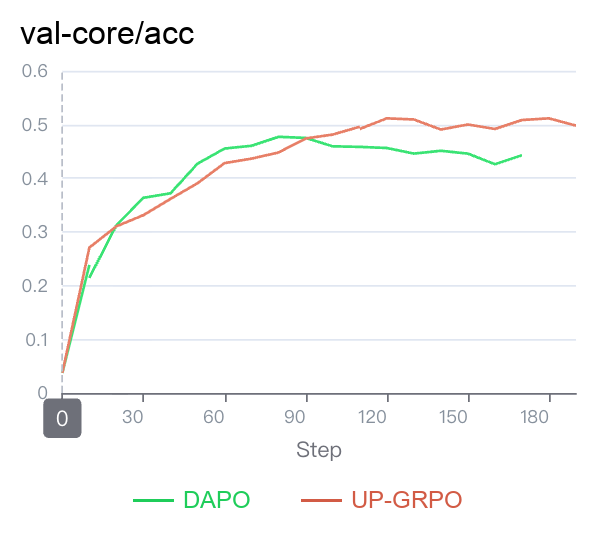
• Peak Performance: UP-GRPO reaches a peak accuracy of 0.5114 (Step 120), whereas the Baseline plateaus early at 0.4770. This is a remarkably significant improvement (+3.44% absolute gain) given the sheer difficulty of AIME problems. Removing the positive clip clearly allows the model to escape suboptimal local minima and confidently memorize correct, complex mathematical reasoning patterns that the baseline algorithm forces it to ignore.

2. KL Divergence: Surprisingly Stable

A common theoretical concern is that unclipped updates will cause the policy to drift uncontrollably (spiking KL divergence). However, Figure 2 (KL Curve) shows UP-GRPO’s KL divergence remains completely stable, often sitting slightly lower than the baseline.

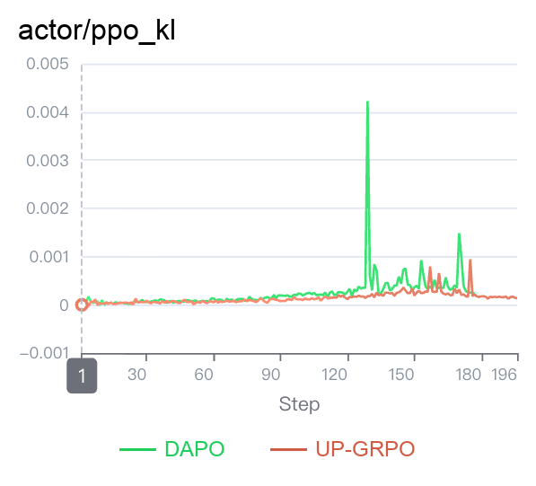
• Why? Because we strictly enforce the clip/trust-region for negative advantages ($A_t \le 0$), “bad” explorations are still heavily constrained. “Good” explorations ($A_t > 0$), while unclipped, naturally pull the model toward high-reward, fundamentally correct regions of the landscape, preventing chaotic drift.

3. Entropy & Early Stopping

Figure 3 (Entropy Curve) reveals a striking differences between UP-GRPO and standard GRPO on their policy entropy curves. While standard GRPO tends to plateau at a lower entropy level in the later stages of training, UP-GRPO exhibits a significant and sustained surge.

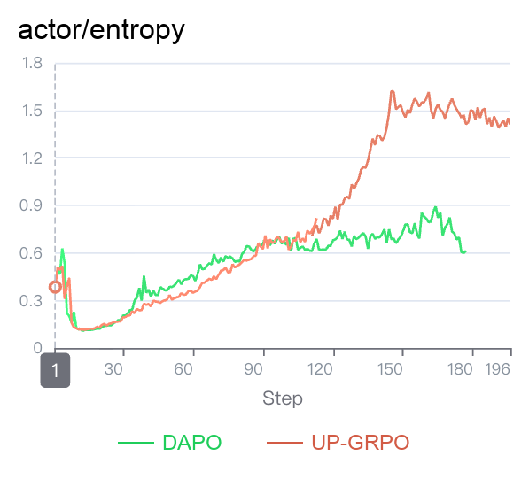
The secret behind this ‘entropy boost’ is UP-GRPO’s elegant asymmetric loss design. By removing the clipping constraint strictly for positive advantages ($A > 0$), UP-GRPO allows the model to aggressively update its policy whenever it discovers exceptionally high-quality, novel responses. Standard GRPO artificially caps the reward for these good explorations, which often forces the model into a narrow probability distribution—a phenomenon known as ‘mode collapse’. In contrast, UP-GRPO’s unbounded positive reinforcement encourages the model to distribute its probability mass across a wider variety of excellent tokens. For the end user, this higher entropy translates to a language model that is not only highly aligned but also remarkably diverse, creative, and resistant to repetitive, formulaic outputs.

6. Conclusion

UP-GRPO is a minimalist yet incredibly powerful algorithmic upgrade for reasoning models. By mathematically restructuring positive advantages into Advantage-Weighted SFT—while retaining standard GRPO trust regions for negative advantages—UP-GRPO perfectly aligns with human learning intuition: reinforce success confidently, but correct failure cautiously.

Our experiments prove that UP-GRPO not only outperforms standard GRPO in mathematical reasoning accuracy but also serves as an elegant theoretical fix for the train-inference routing mismatch that plagues MoE architectures.

Appendix: Implementation Details (PyTorch)

The following PyTorch snippet demonstrates the core implementation of the UP-GRPO policy loss. This implementation is designed to be a drop-in replacement for the standard policy loss in verl.

The key logic resides in the conditional branching: for tokens with $A_t > 0$, we bypass the importance ratio and clipping entirely, using a direct likelihood-based loss ($-\log \pi_\theta \cdot A_t$).

import torch
import torch.nn.functional as F

def compute_policy_loss(old_log_prob,
                        log_prob,
                        advantages,
                        response_mask,
                        cliprange=None,
                        cliprange_low=None,
                        cliprange_high=None,
                        clip_ratio_c=3.0,
                        loss_agg_mode="token-mean"):
    """Adapted from https://github.com/huggingface/trl/blob/main/trl/trainer/ppo_trainer.py#L1122
    Args:
        old_log_prob: `(torch.Tensor)`
            shape: (bs, response_length)
        log_prob: `(torch.Tensor)`
            shape: (bs, response_length)
        advantages: `(torch.Tensor)`
            shape: (bs, response_length)
        response_mask: `(torch.Tensor)`
            shape: (bs, response_length)
        cliprange: (float)
            The clip range used in PPO. See https://arxiv.org/abs/1707.06347
        cliprange_low: (float)
            The lower clip range used in PPO.
        cliprange_high: (float)
            The higher clip range used in PPO.
        clip_ratio_c: (float) default: 3.0
            The lower bound of the ratio for dual-clip PPO, See https://arxiv.org/pdf/1912.09729
        loss_agg_mode: (str) choices: "token-mean" / "seq-mean-token-sum" / "seq-mean-token-mean"
            "token-mean" is the default behavior        

    Returns:
        pg_loss: `a scalar torch.Tensor`
            policy gradient loss computed via PPO
        pg_clipfrac: (float)
            the fraction of policy gradient loss being clipped
        ppo_kl: (float)
            the estimated KL divergence between the latest updating policy and the old sampling policy
        pg_clipfrac_lower: (float)
            the fraction of policy gradient loss being clipped when the advantage is negative
    """
    assert clip_ratio_c > 1.0, f"The lower bound of the clip_ratio_c for dual-clip PPO should be greater than 1.0, but get the value: {clip_ratio_c}."



    negative_approx_kl = log_prob - old_log_prob
    ratio = torch.exp(negative_approx_kl)
    
    ppo_kl = verl_F.masked_mean(-negative_approx_kl, response_mask)

    # 1. POSITIVE PATH (A > 0): Unbounded Reinforcement (AW-SFT)
    # We treat these as "golden" signals that the model should maximize without constraints.
    pg_losses_pos = -advantages * log_prob

    # 2. NEGATIVE PATH (A <= 0): Standard Clipped GRPO
    # Protects against policy collapse and keeps the update within the trust region.
    pg_losses1_neg = -advantages * ratio
    if cliprange_low is None:
        cliprange_low = cliprange
    if cliprange_high is None:
        cliprange_high = cliprange
    pg_losses2_neg = -advantages * torch.clamp(ratio, 1 - cliprange_low, 1 + cliprange_high)
    
    clip_pg_losses1_neg = torch.maximum(pg_losses1_neg, pg_losses2_neg)
    
    pg_losses3_neg = -advantages * clip_ratio_c
    
    clip_pg_losses2_neg = torch.min(pg_losses3_neg, clip_pg_losses1_neg)
    


    # Note: This `torch.where` is kept to strictly align with the standard GRPO loss implementation.
    # Logically, it is redundant and could be simplified to: `pg_losses_neg = clip_pg_losses2_neg`.
    # Because when `advantages == 0`, both `clip_pg_losses1_neg` and `clip_pg_losses2_neg` are exactly 0,
    # and when `advantages > 0`, the value will be overridden by `pg_losses_pos` in the next `torch.where`.
    pg_losses_neg = torch.where(advantages < 0, clip_pg_losses2_neg, clip_pg_losses1_neg)

    pg_losses = torch.where(advantages > 0, pg_losses_pos, pg_losses_neg)

   
    pg_loss = agg_loss(loss_mat=pg_losses, loss_mask=response_mask, loss_agg_mode=loss_agg_mode)


    # (Logging) Calculate clipping fraction only for the negative path
    neg_adv_mask = (advantages <= 0).float() * response_mask
    
    clip_frac_tensor = torch.gt(pg_losses2_neg, pg_losses1_neg).float()
    pg_clipfrac = verl_F.masked_mean(clip_frac_tensor, neg_adv_mask)

    lower_clip_frac_tensor = torch.gt(clip_pg_losses1_neg, pg_losses3_neg).float()
    pg_clipfrac_lower = verl_F.masked_mean(lower_clip_frac_tensor, neg_adv_mask)

    return pg_loss, pg_clipfrac, ppo_kl, pg_clipfrac_lower

💡 A Mathematical Note: Loss Magnitude vs. Gradient Scale

A sharp-eyed reader inspecting the code above might notice a numerical discrepancy. The positive path calculates loss using log_prob (which is typically a negative value with a larger absolute magnitude, e.g., $-2.0$ to $-10.0$), whereas the negative path uses ratio (which is tightly centered around $1.0$).

A natural question arises: Doesn’t mixing these vastly different numerical scales in a single loss tensor and aggregating them destabilize training?

The beautiful answer is no, because deep learning optimizers (like Adam) operate on gradients, not raw loss scalars. Let us examine the gradients for both paths:

• Positive Path Gradient ($A_t > 0$): \(\nabla_\theta \mathcal{L}_{Pos} = \nabla_\theta (-A_t \log \pi_\theta) = -A_t \cdot \nabla_\theta \log \pi_\theta\)
• Negative Path Gradient ($A_t \le 0$): \(\nabla_\theta \mathcal{L}_{Neg} = \nabla_\theta \left(-A_t \frac{\pi_\theta}{\pi_{old}}\right) = -A_t \frac{1}{\pi_{old}} \nabla_\theta \pi_\theta = -A_t \underbrace{\left(\frac{\pi_\theta}{\pi_{old}}\right)}_{r_t} \nabla_\theta \log \pi_\theta = -A_t \cdot r_t \cdot \nabla_\theta \log \pi_\theta\)

Because the trust-region mechanism inherently restricts the policy update such that $r_t \approx 1$, the scale of the gradients is perfectly, continuously aligned across the $A_t = 0$ boundary. Despite the raw forward-pass loss values residing in completely different numerical manifolds, their backward-pass gradient signals flow together seamlessly.